
Abstract
The transient response of resistor-capacitor (RC) circuits under direct current (DC) excitation represents a fundamental topic in electrical engineering and applied physics. This article provides a rigorous, and fully derived of the charging and discharging processes, emphasizing formulas, physical interpretation, and engineering relevance.
Introduction
RC circuits are first-order linear dynamic systems whose transient behavior arises when a switch connects or disconnects a DC source. These processes describe how energy is stored and released in a capacitor and are mathematically governed by differential equation of the first order with constant coefficients.
Two key regimes are analyzed:
- Charging (switch ON)
- Discharging (switch OFF)
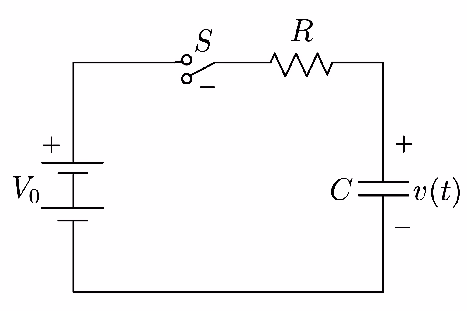
Mathematical Model of the RC Circuit
Applying Kirchhoff’s Voltage Law (KVL):
V0 = vR(t) + vC(t)
Using:
vR(t) = R * i(t)
i(t) = dq/dt = C * (dvC/dt)
Substitute:
V0 = R * C * (dvC/dt) + vC
Charging Process (Switch Closing at t = 0)
Differential Equation
Initial condition:
vC(0) = 0
Governing equation:
R * C * (dvC/dt) + vC = V0
Step-by-Step Derivation
Rearrange:
dvC/dt = (1 / (R * C)) * (V0 – vC)
Separate variables:
dvC / (V0 – vC) = dt / (R * C)
Integrate:
– ln(V0 – vC) = t / (R * C) + K
Solve:
V0 – vC = A * e^(-t/(R*C))
Apply initial condition:
vC(0) = 0 → A = V0
Final Voltage Expression
vC(t) = V0 * (1 – e^(-t/(R*C)))
Current Expression
i(t) = C * (dvC/dt)
Result:
i(t) = (V0 / R) * e^(-t/(R*C))
Physical Interpretation
- At t = 0:
vC = 0, i = V0 / R
- At t → ∞:
vC → V0, i → 0
- Capacitor behaves:
- Initially as a short circuit
- Eventually as an open circuit
Time Constant (Key Parameter)
τ = R * C
Meaning:
- At t = τ:
vC ≈ 0.632 * V0
Hence comes the definition of the time constant, which is the time for which the voltage (in general, the signal) reaches 63.2% of its maximum value.
- At t = 5 * τ:
vC ≈ 0.993 * V0
Discharging Process (Switch Opening)
Initial condition:
vC(0) = V0
Differential Equation
R * C * (dvC/dt) + vC = 0
Solution
Rearrange:
dvC/dt = -vC / (R*C)
Separate variables:
dvC / vC = -dt / (R*C)
Integrate:
ln(vC) = -t/(R*C) + K
Solve:
vC = A * e^(-t/(R*C))
Apply initial condition:
A = V0
Final Voltage Expression
vC(t) = V0 * e^(-t/(R*C))
Current Expression
i(t) = -(V0 / R) * e^(-t/(R*C))
Interpretation
- Voltage decreases exponentially
- Current reverses direction
- Energy is dissipated as heat in resistor
Unified General Solution
All first-order systems can be expressed as:
x(t) = x_inf + (x0 – x_inf) * e^(-t/τ)
Where:
τ = R * C
Energy Analysis
Energy stored in capacitor:
W = (1/2) * C * V0^2
Important result:
- 50% energy stored
- 50% dissipated in resistor during charging
Engineering Applications
- Low-pass filters
- Timing circuits
- Pulse shaping networks
- Power supply smoothing
- Communication systems
Advanced Insight: Exponential Nature
The exponential response:
e^(-t/(R*C))
appears due to:
- Linear differential equation (differential equation of the first order with constant coefficients)
- Energy storage element (capacitor)
- Dissipative element (resistor)
This same mathematical structure appears across:
- Thermal systems
- Mechanical damping
- Population decay models
Conclusion
The transient response of RC circuits to DC switching is one of the most elegant examples of first-order system dynamics. Through rigorous derivation and interpretation, we see how exponential laws emerge naturally from physical principles.
Mastery of these equations enables:
- Accurate circuit design
- Efficient signal analysis
- Deep understanding of dynamic systems
Differential equation:
R * C * (dvC/dt) + vC = V0
can be solved in another way:
After dividing by R * C we get:
dvC/dt + vC / (R * C) = V0 / (R * C)
The solution of this differential equation is obtained as the sum of the solution of the corresponding homogeneous equation and the particular solution.
In the first case, the equation should be solved:
dvC/dt + vC / (R * C) = 0
This means that:
dvC/dt = – vC / (R * C)
so it is:
dvC/vC = -dt/(R * C)
After applying the integral:
ln (vC) = -t / (R * C) + ln (C)
ln (vC) – ln (C) = -t / (R * C)
ln (vC/C) = -t / (R * C)
vCh = C * e^(-t/(R*C))
To determine the particular solution, the assumed solution of the differential equation should be given. It is easy to conclude that it will be vC = K (K is a constant). This means that dvC/dt = 0, so K = V0 or vCp = V0, so vC = C * e^(-t/(R*C)) + V0.
Based on the initial conditions vC = 0, t = 0, it is obtained that C = -V0, so:
vC(t) = V0 * (1 – e^(-t/(R*C)))
An interesting observation can be made from the expression
vC(t) = V₀ · (1 − e^(−t/(RC)))
Since the exponent of an exponential function must be dimensionless, the product RC must have the dimension of time.
Indeed,
R = V/I
C = Q/V
therefore
RC = (V/I) · (Q/V) = Q/I
Since Q = It, it follows that
RC = (It)/I = t
Thus, the time constant τ = RC is not merely a mathematical parameter – it is physically a quantity with the dimension of time.